Emaraic

Weakly Supervised Object Detection In Practice

Introduction

Convolution neural networks (CNN) have been commonly chosen for classification and localization tasks. Although these tasks require data collecting for training, data collecting for classification task is easier and more available than the one for object detection task which requires an intensive task of annotating every object in a given image. For this reason, many works move towards exploiting CNN classification models for object detection task without the guidance of bounding box annotations of objects, which is known as weakly-supervised object localization.
One of the proposed approaches was demonstrated by Researchers from MIT to provide a simple technique for exploiting an existent classification model to perform object localization and also identifying parts of the image which have the largest contribution in discrimination task using a Global Average Pooling (GAP) layer to generate a Class Activation Map (CAM)^[1].
In this post, we will explain this method along with Global Average Pooling and Class Activation Map. And then how to apply this technique to make a classification network performs both object classification and object localization in a single forward-pass.

Requirements:

1. Pytorch and torchvision.
2. Opencv, Pillow and Numpy.

Global Average Pooling

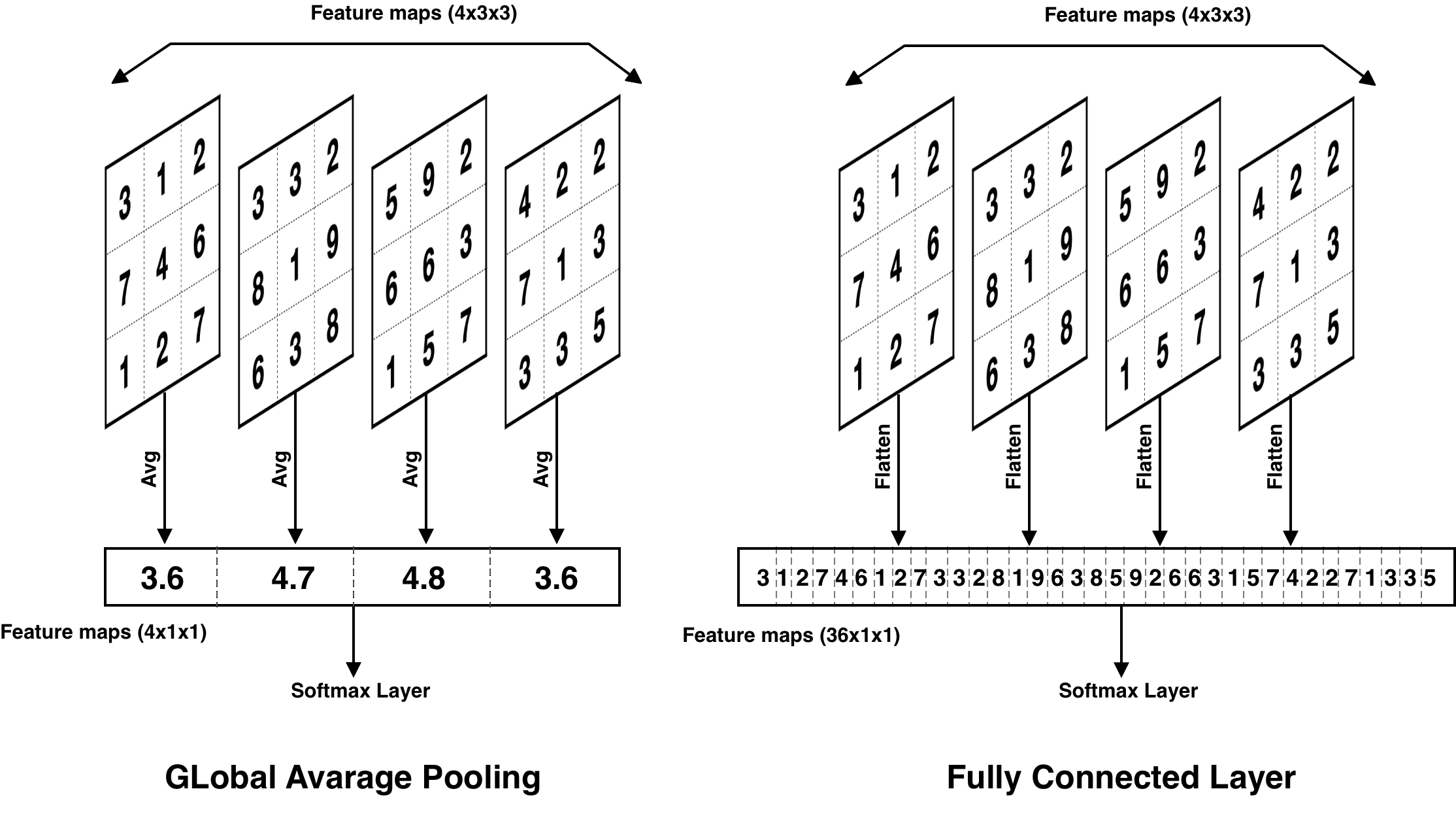
Convolutional neural networks usually contain a successive series of convolution and pooling layers to generate feature maps which must be an efficient representative for the input image. Then these feature maps are flattened and fed to fully connected layers to classify input images. This design was common till the proposed design in Network in Network (NIN)^[2] model, which replaces the fully connected layers with Global Average Pooling layer. The avoidance of using fully connected layers is a result of their proneness to overfit as they have the largest number of trainable parameters in the network, resulting in a reduction in the generalization ability of the network. For example, in Resnet18, the last convolution layer produces feature map of size of 512x7x7 (512 feature map each with size 7x7), consider we want to feed them to a fully connected layer to classify the current 3 classes, so the total number of trainable parameters is (7x7x512x3) + 3 = 75267.
Instead of using fully conned layers, networks include a Global Average Pooling layer after the last convolution layer to create by taking the average of each generated feature map, as shown in figure 2. Using the previous example, the last feature maps 512x7x7 passed through global average pooling resulting a vector of 512x1x1, so the total number of trainable parameters is (1x1x512x3) + 3 = 1539.

Advantages of using Global Average Polling can be summarized as:

1. It reduces the number of trainable parameters which reduces the overfit error.
2. It is more robust to spatial translations (for example, the location of an object in an image) of the input as it averages all features maps across all the spatial positions.
3. it allows networks to accept images with different size as Fully Convolution Networks, for example, consider an input image with size 224x224 generates final feature maps of size 7x7x512 which will be 1x1x512 after apply global average pooling, if we change the size to 448x448, the final feature maps will have size 14x14x512 which will be also 1x1x512 after applying global average pooling. This resulting in a fixed length of a vector to be fed to the softmax layer.

Class Activation Map

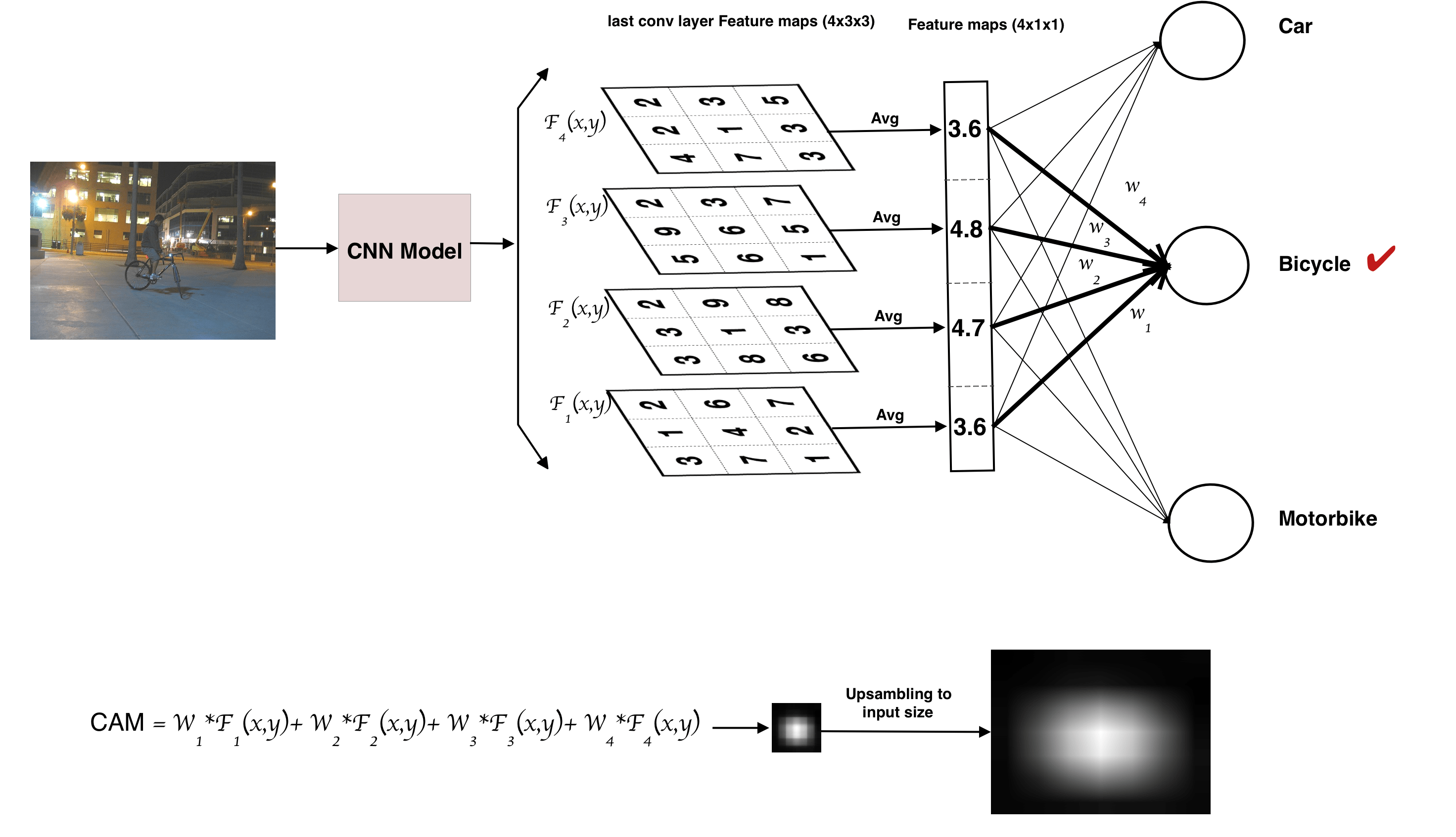
Class activation map is a weighted features maps generated for each image to indicate the discriminative regions used by the CNN to identify the class this image belongs to. To describe the procedure to generate CAM, let's first for simplicity, suppose we have a network to classify a given image to 3 classes (Car, Bicycle, and Motorbike). It generates feature maps F_k(x,y) where k is the number of kernels after the last convolution. The procedure can be described with the aid of figure 2 as follows:

1. Forward a given image to the network and get the index of the prediction class, suppose it is predicted as a bike.
2. A weighted sum of feature maps is computed by multiplying each feature map (F_k(x,y)) by correspondent weights between the output node of predicted class (Bicycle node) and the output of global average pooling (W₁, W₂, W₂, W₄) and summing the result, as the equation
   Cam=W₁*F₁(x,y) + W₂*F₂(x,y) + W₃*F₃(x,y) + W₄*F₄(x,y)
3. Upsample the result from the previous step to the input image resolution.

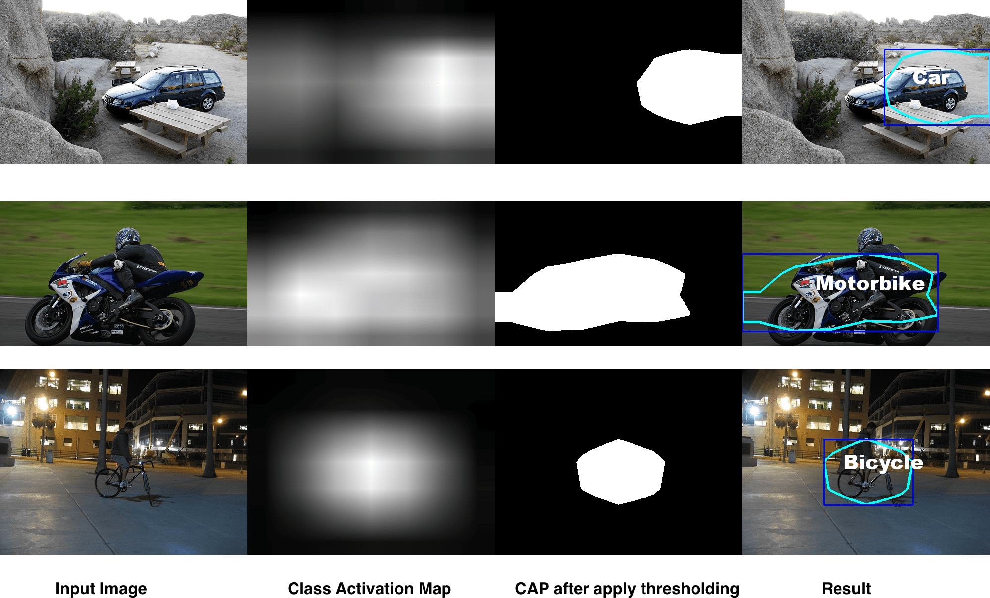
Generating Bounding Box from CAM

Till now, we do not have a bounding box for an existent object in a given image from CAM. To get it, we apply simple post-processing steps including, thresholding the CAM image and find contours (boundaries) of including objects as shown in figure 3.

Source Code

Training

We will use a pre-trained Resnt18 to be trained on a classification dataset which has a 3 classes Car, Bicycle, and Motorbike, from a kaggle competition (here). All you need is to download the dataset from (here) and run the training script train.py via this command.

 python train.py --dataset_train_path /path/to/train --classes 3

Demo

After finishing the training, you can test your classification model as an object detection one, by running demo.py script. All you need is to provide it by, a model weights path, an input image path, and the number of classes of the model such as the following command.

 python demo.py --model_path path/to/model/weights --image_path /path/to/image --numclasses 3

Notes

1. You can skip the training, if you want to test the demo code directly, just run demo.py script with default values as I provided the pre-trained weights and test samples in the source code repo.
2. You can get the source code from https://github.com/tahaemara/weakly-supervised-detection.

References

• Zhou, Bolei, et al. "Learning deep features for discriminative localization". Proceedings of the IEEE conference on computer vision and pattern recognition. 2016.
• Lin, Min, Qiang Chen, and Shuicheng Yan. "Network in network". arXiv preprint arXiv:1312.4400 (2013).